Made by
Neel Shirish Anap, anap.n@northeastern.edu
Prayansh Maheshwari, maheshwari.pray@northeastern.edu
- Problem Setting
- Project Goal
- Data Description
- Data Exploration and Visualization
- Data Pre-processing
- Machine Learning Models
- Results
1. Problem Setting
Marketing analytics is the study of data to evaluate the effectiveness of marketing initiatives. Businesses can improve their marketing campaigns, comprehend what motivates consumer behavior, and maximize their return on investment. In this project, we’ll examine whether a customer bought a product as a result of some website features. From a marketing perspective, it would be very advantageous to analyze this trend and forecast product sales because it would assist the business in making various decisions, such as deciding whether to stock the product or plan for discounts.
2. Project Goal
A specific business that maintains a website to sell its goods in a virtual marketplace wants to forecast when a product will be bought. Finding patterns and similarities between customers who have purchased the product and those who have not will help us solve this issue by grouping the two groups of customers into clusters. Numerous elements or characteristics that the business has learned about from its website ultimately affect the customer’s choice to buy the product. These are the variables that we intend to use to predict and build a dependency on a purchase.
3. Data Description
The dataset for this project is taken from the UCI Machine Learning Repository: Online Shopper’s Purchase Intention. The dataset containing the site’s statistics is called “Online Shoppers’ Purchase Intention.” The dataset has 18 columns and approximately 12K rows. There are 10 numerical and 8 categorical variables. The target variable is a string variable named “Purchased,” which marks whether the customer purchased a product or not.
4. Data Exploration and Visualization
To make sure the dataset is complete, the null entries are examined first. Our dataset is found to have no missing or null values, making it suitable for use in machine learning tasks.

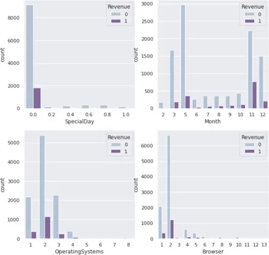
4.1 Categorical Variables
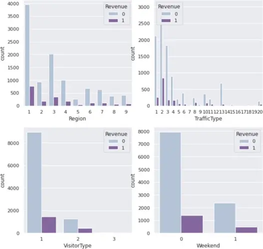
Distribution is presented for categorical variables with respect to the target variable “Revenue” (Product bought or not). Each categorical variable’s impact on the customer’s choice is shown. The graphs below show that the Special Day category has no bearing on the target variable. Looking at the months, we can observe that May, November, and December have larger sales of products than the other months, which may be related to the holiday shopping season. Users only utilize a small number of operating systems and browsers, and as a result, a small number of them display the target variable response. The charts below show that regions and traffic categories 1 to 4 have the highest likelihood of making a purchase. Compared to other visitor types, visitor type 1 has the highest conversion potential. The graph shows that weekday users of the site had the high probability of making a purchase, indicating that the weekend does not have a significant impact on customer purchases.
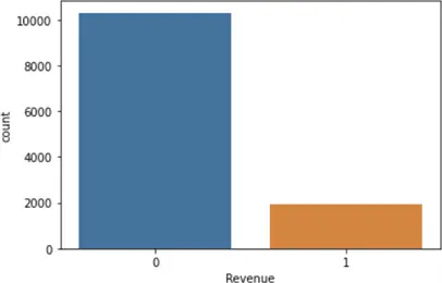
We can see the percentage of clients who buy or don’t buy a product from the plot below. Our data is very imbalanced, with more than 80% being 0 and 20% being 1.
4.2 Numerical Variables
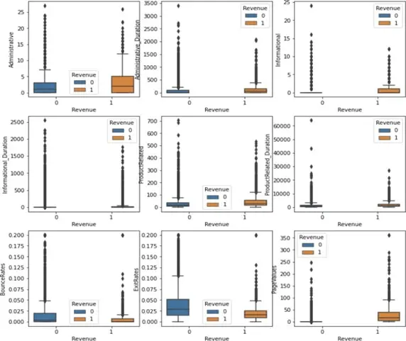
Summary of the numerical variables. We can see that most of the variables are right skewed.

Similar to how most real-world data is right skewed, boxplots are also produced for numerical variables, showing that our data lacks a distinct center.
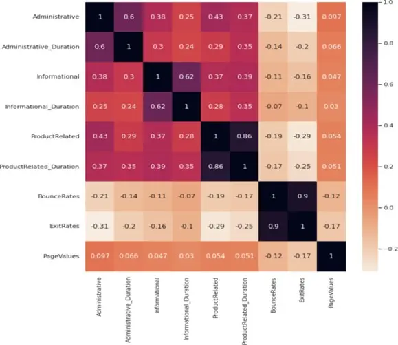
To determine the correlation between the numerical variables, we have also created a correlation heatmap. We can see high correlation between Administrative and Administrative_duration, Informational and Informational_duration, ProductRelated and ProductRelated_duration, and BounceRates and ExitRates. And few columns showing negative correlation as well.
5. Data Pre-processing
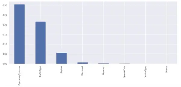
For the purpose of choosing features for categorical variables, the chi square test has been used. First, the categorical data was transformed into nominal categories before the chi test was performed. From the graph below we can he variables OperatingSystems and TrafficType has a p value larger than 0.05, hence these variables are dropped from the dataset.
Following that, we examined the skewness of the numerical variables. The majority of the variables are clearly severely skewed, as can be seen in the table below. To fix this skewness in the dataset, we applied the square root technique.
Skewness Before:
| Attribute | Skewness Before | Skewness After |
|---|---|---|
| Administrative | 1.941723 | 0.625303 |
| Informational | 4.014173 | 1.933381 |
| ProductRelated | 4.333419 | 1.5033354 |
| BounceRates | 3.162425 | 1.715256 |
| PageValues | 6.350983 | 2.515993 |
| Administrative_Duration | 5.592152 | 1.527806 |
| Informational_Duration | 7.540291 | 3.419129 |
| ProductRelated_Duration | 7.253161 | 1.412977 |
| ExitRates | 2.234645 | 1.211128 |
Following that, we removed the highly correlated columns from the dataset based on the correlation plot. The categorical attributes were then subjected to One hot encoding, resulting in the addition total of 47 columns. The data was divided into training (75%) and test (25%) sets. After this, as our dataset was imbalanced, we performed SMOTE technique of oversampling the minority class which in terms of our dataset was Revenue as 1. Then, before employing any machine learning models, the training data was standardized. The test data was then converted using the training data mean and standard deviation. Skewness before Skewness after
6. Machine Learning Models
The following models have been implemented:
- Logistic Regression
- Naïve Bayes
- Neural Networks
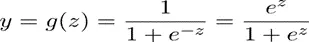
6.1 Logistic regression
Logistic Regression is the most common type of classification model which calculates some optimal parameters. When the input is multiplied by these learned optimal parameters, we get a binary output, 0 or 1 in this case.
The model’s performance is determined by the cost function. It is employed to gauge how closely the model’s predictions match the actual results. The cost can be computed numerically as follows for specific “m” observations:
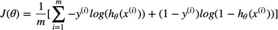
Then, we used the following parameters to train our model: Maximum iterations are 5000, Tolerance is 0.00005, and Alpha is 0.00001. Below is the graph that was produced by the gradient descent algorithm. As the number of iterations rises, the error is depicted on the graph.
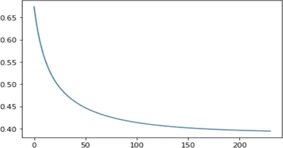
We estimated the result for training error using the weights, and we calculated cutoff vs sensitivity/accuracy to select the best cutoff. These are the outcomes:
| Cutoff | Sensitivity | Accuracy | |
|---|---|---|---|
| 0 | 0.10 | 0.979555 | 0.812812 |
| 1 | 0.20 | 0.937301 | 0.907542 |
| 2 | 0.40 | 0.870286 | 0.927533 |
| 3 | 0.60 | 0.781009 | 0.887778 |
| 4 | 0.80 | 0.668560 | 0.833371 |
| 5 | 0.95 | 0.414357 | 0.706951 |
In order to achieve a better balance between sensitivity and accuracy, we choose to utilize a cutoff of 0.4. The following outcomes are obtained after applying our trained model to our testset:
Confusion Matrix:
| Predicted 1 | Predicted 0 | |
|---|---|---|
| Actual 1 | 1419 | 24 |
| Actual 0 | 171 | 105 |
Sensitivity and Accuracy
| Sensitivity | Accuracy |
|---|---|
| 0.8865619546247818 | 0.3804347826086957 |
6.2 Gaussian Naïve Bayes
The Gaussian Naive Bayes model classifies a new data point based on the data available. It is the simplest type of model where the calculations are based on probabilities and likelihoods.
The following is the Bayes Theorem calculation in its simplest version. Where the marginal probability of the occurrence P(A) is referred to as the prior and the probability that we are interested in computing P(A|B) is called the posterior probability.
P(A|B) = P(B|A) * P(A) / P(B)
The likelihood of a predictor for a given class is its probability. The number of examples (rows) in the training dataset divided by the proportion of observations with the class label can be used to determine the prior.
P(yi) = examples with yi / total example
To determine if the model is overfitting or not, we trained the priors for the training set and produced predictions for both the training and test sets.
Training Dataset:
Confusion Matrix:
| Predicted 1 | Predicted 0 | |
|---|---|---|
| Actual 1 | 3324 | 4427 |
| Actual 0 | 1213 | 6538 |
Sensitivity and Accuracy
| Sensitivity | Accuracy |
|---|---|
| 0.843504063991743 | 0.6361759772932525 |
Testing Dataset:
Confusion Matrix:
| Predicted 1 | Predicted 0 | |
|---|---|---|
| Actual 1 | 1086 | 1460 |
| Actual 0 | 229 | 277 |
Sensitivity and Accuracy
| Sensitivity | Accuracy |
|---|---|
| 0.5474308300395256 | 0.44659239842726084 |
6.3 Neural Networks
A neural network model tries to imitate the human brain. There are layers of neurons , which are essentially gates where some calculation takes place. Each neuron has a weight and a bias.
Mathematically the calculation at a node is given by:
a1 = wi*xi + bi, where wi is weight and bi is bias
The procedure of back propagation is used to calculate the gradient of neural network parameters. The method essentially traverses the network from the output to the input layer in reverse order using the chain rule from calculus to update weights and biases thereby introducing learning factor in the model.
The error function’s gradient with regard to the weights and biases is calculated,
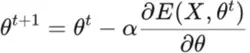
The mean squared error serves as the error function in traditional backpropagation.
With two hidden layers (16, 8) and an output layer with a sigmoid activation function, we created neural networks using Keras. We used relu for the hidden layer’s activation function, the Adam optimizer for loss, and binary cross entropy loss for loss. We ran the model for 100 epochs and observed that the training accuracy and validation accuracy were almost at constant values.
| Cutoff | Sensitivity | Accuracy | |
|---|---|---|---|
| 0 | 0.10 | 0.989096 | 0.930713 |
| 1 | 0.20 | 0.975239 | 0.953090 |
| 2 | 0.40 | 0.955929 | 0.960813 |
| 3 | 0.60 | 0.937756 | 0.959109 |
| 4 | 0.80 | 0.904362 | 0.950136 |
| 5 | 0.95 | 0.858701 | 0.929010 |
For testing, we decided to keep the cutoff as 0.4 and we got the following results:
Confusion Matrix:
| Predicted 1 | Predicted 0 | |
|---|---|---|
| Actual 1 | 1373 | 70 |
| Actual 0 | 84 | 192 |
Sensitivity and Accuracy
| Sensitivity | Accuracy |
|---|---|
| 0.6956521739130435 | 0.910413030831879 |
Training accuracy vs validation accuracy
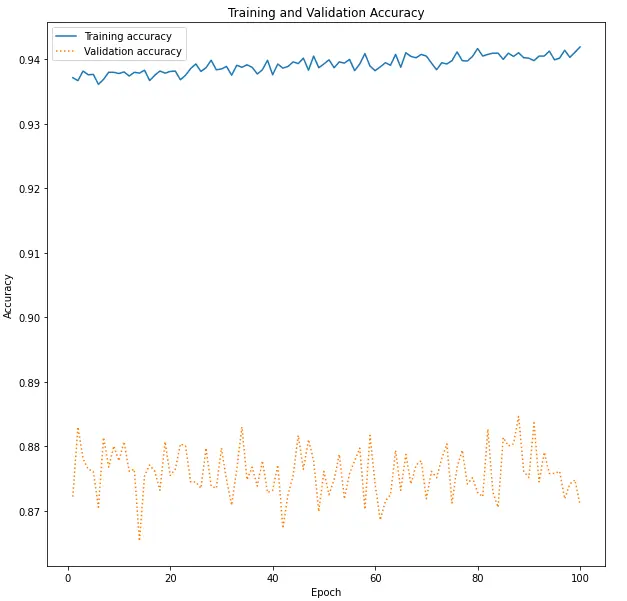
The validation accuracy is lower than the training accuracy indicating that the model is overfitting on training data. To solve this problem , we tried to implement regularization techniques in Neural Network by adding a L2 norm and dropout layers. Although it did not affect the accuracy scores, it did lower the accuracy of model on testing data which is undesirable.
7. Results
Since the goal of our model is to determine the likelihood that a customer would purchase a product, we must trade off poor specificity for higher accuracy and sensitivity. Classifying a product’s likelihood of purchase is crucial in order to decide whether to invest in targeted marketing initiatives, among other things. Reaching them through marketing may result in more income, even if some consumers who are not going to buy are recognized as potential customers. However, we risk losing potential customer if we incorrectly categorize the customers who are about to make a transaction.
| Model | Cutoff | Sensitivity | Accuracy |
|---|---|---|---|
| Logistic Regression | 0.4 | 0.3804347826086957 | 0.8865619546247818 |
| Gaussian Naive Bayes | - | 0.5474308300395256 | 0.44659239842726084 |
| Neural Network | 0.4 | 0.6956521739130435 | 0.910413030831879 |
Neural Networks provide the highest accuracy and respectable sensitivity according to the metric comparison displayed above. Naive Bayes is the worst model as both its metrics are the lowest.