Monitoring

Outline:

1. Introduction
   
2. Scoping
   
3. Setup on Azure & Databricks(Optional)
   
4. Data
   
5. Modeling
   
6. Deployment
   
7. Monitoring
   
8. Cost Analysis
   

MLFlow Overview in Test Environment

MLFlow is an integral part of our MLOps pipeline, providing model versioning, management, and serving capabilities. This document outlines the key aspects of MLFlow operations within the test environment, detailing version controls, artifact handling, and how to utilize the models within the Databricks environment.

Registered Models in Test Environment

Our MLFlow setup includes several versions of the model, with detailed tracking of experiments and model performance metrics.

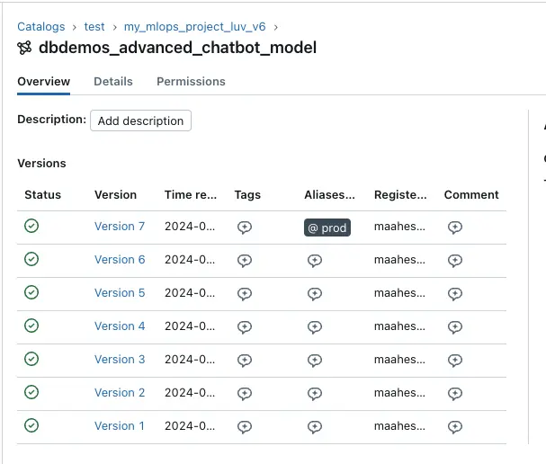
About Version 7

Version 7 of the model is currently in the ready state and is serving predictions. This model incorporates improvements over previous versions and includes comprehensive logging of input and output schemas as well as detailed artifact storage.

Previous Versions

Version 6, which was active before Version 7, is also documented to provide insights into the model’s evolution and basis for improvements.

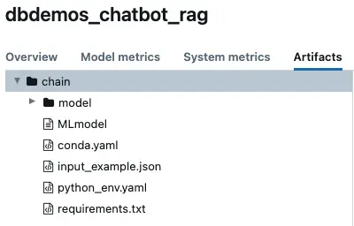
Artifacts and MLmodel File

The artifacts stored in MLFlow provide a detailed breakdown of the model components. The MLmodel file is a key artifact that outlines the model configuration, dependencies, and the environment setup required to run the model.

Artifacts details are shown below:

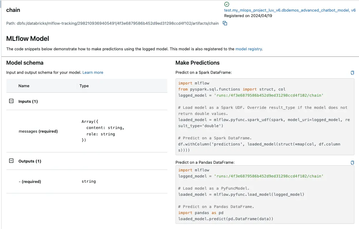
Overall details of Model Schema, MLFlow Model is shown:

Prod Environment Overview

In the production environment, model versioning and management follow a streamlined process tailored for operational stability and performance. This section outlines how models are handled in production within our MLOps setup using MLFlow.

Models in Production

Once the production models are fully operational, they serve the advanced functionalities of a chatbot, which is a significant component of our service offerings. The models in production are managed with distinct versioning practices to ensure stability and traceability.

Model Registry and Versioning

Model versioning in production is handled through the MLFlow model registry, where each model version is meticulously documented and stored. Below are the details of a typical model setup in production:

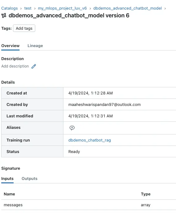
Training and Artifacts

Each model version in production is linked to a specific training run, allowing us to trace back to the experimental setups and configurations. This traceability ensures that any deployed model can be audited and validated against its training parameters and outcomes.

• Training Run: dbdemos_chatbot_rag
• Artifact Path: This path provides access to all relevant artifacts associated with the model, including the MLmodel configuration files, environmental dependencies, and the actual model data.

Accessing and Managing Models

To access and manage the deployed models in production:

1. Navigate to the MLFlow model registry via the Databricks workspace.
2. Select the dbdemos_advanced_chatbot_model to view all versions and their details.
3. Each model version can be examined for its input and output signatures, artifacts, and the exact time of creation and last modification.

Model Version Rollback

To revert to a prior version of a model in a production environment, you can follow the procedure outlined below:

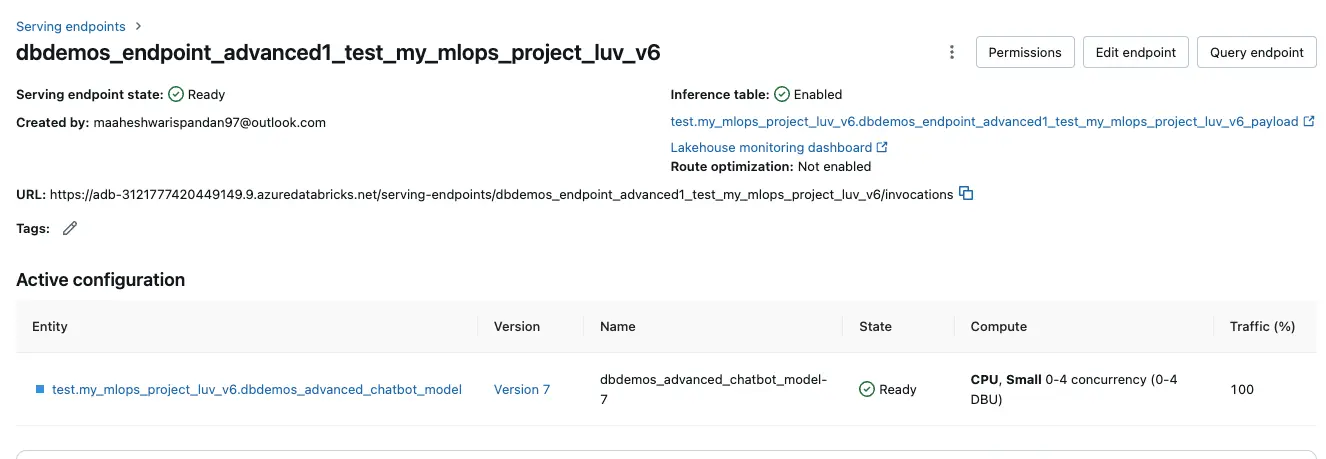
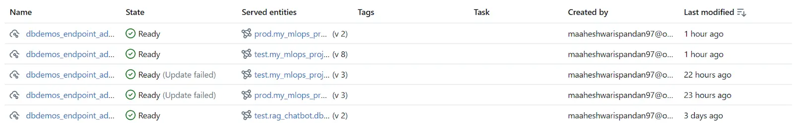
Step 1: Navigate to the Serving Section

Access the “Serving” section via the left sidebar in Databricks, which displays a list of all active serving endpoints.

Step 2: Select the Deployed Model

Identify and select the model currently deployed in production. This will present you with a screen similar to the following:

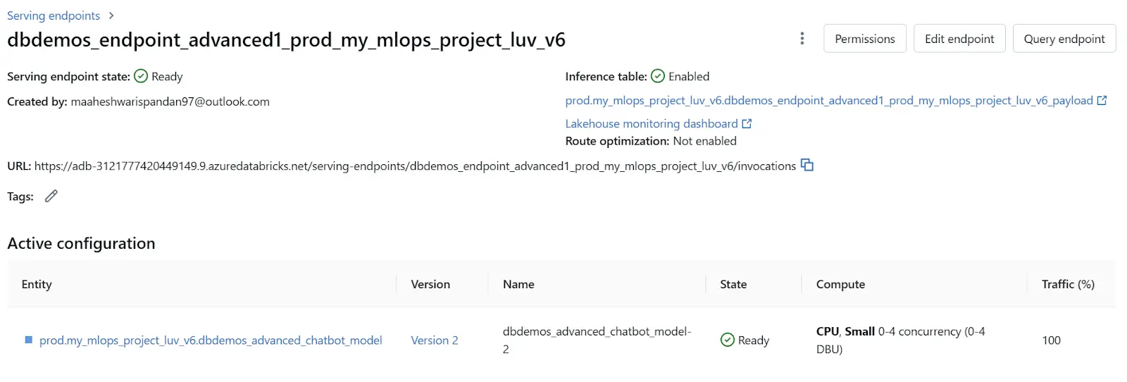
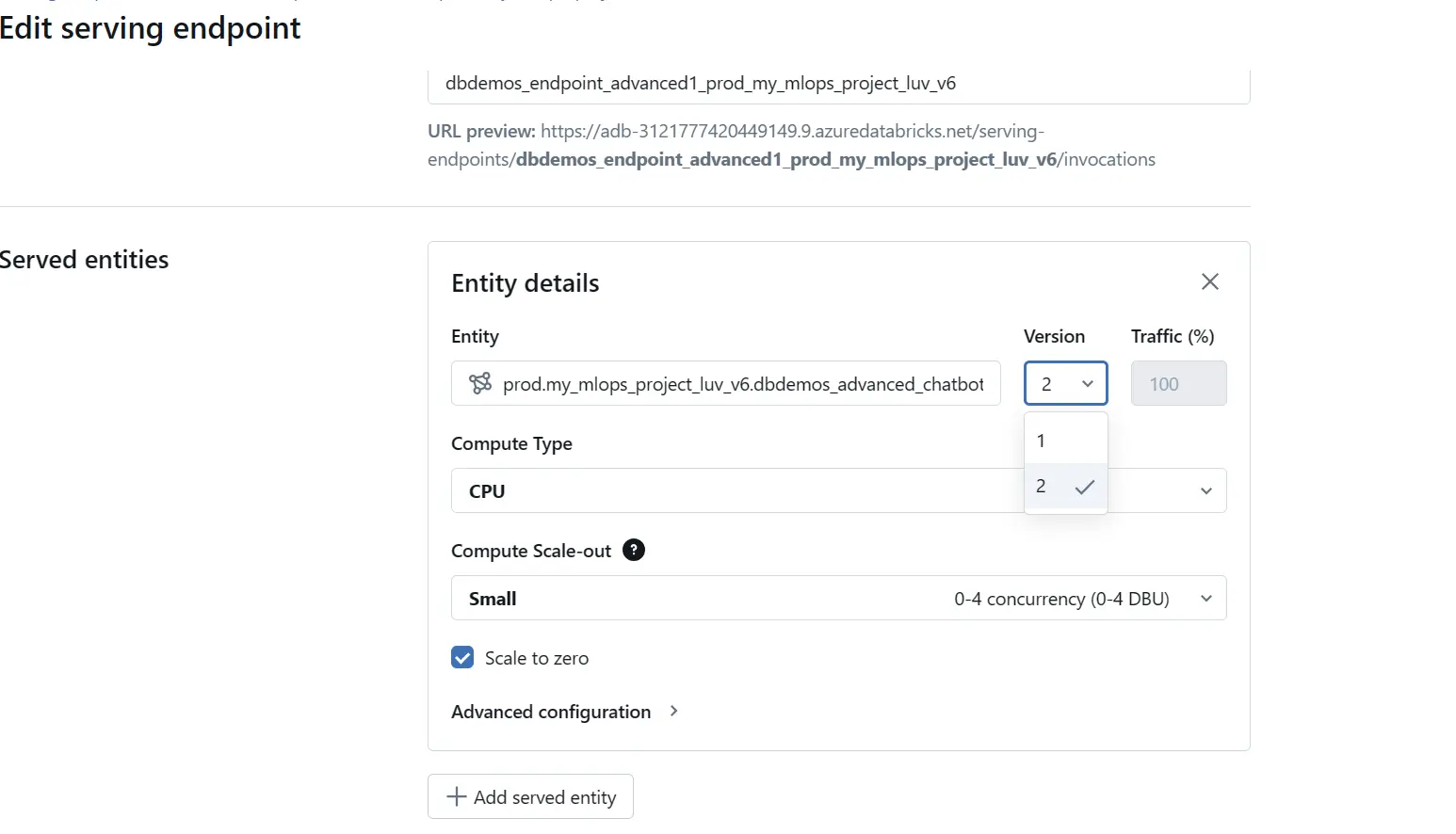
Step 3: Edit Endpoint

In the upper-right corner, click on “Edit endpoint”. Within this area, locate the “Served entities” section, which includes a version dropdown menu. This menu allows you to view and select from previously deployed model versions. Choose the desired version and confirm the rollback by clicking “Update”.

Inference Table Analysis using Databricks Lakehouse Monitoring

Inference Table Analysis using Databricks Lakehouse Monitoring Databricks Lakehouse Monitoring automatically builds a dashboard to track your metrics and their evolution over time. We have manually built other visualizations, here are some of them.

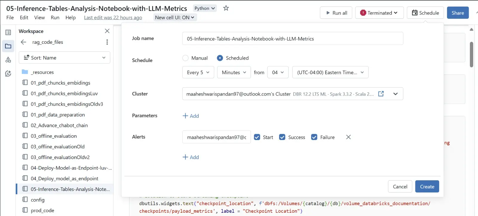
Here we are creating a job scheduling trigger, which will trigger our inference tables every 5 minutes, which generates the evaluation matrices that are being used for further in-depth analysis.

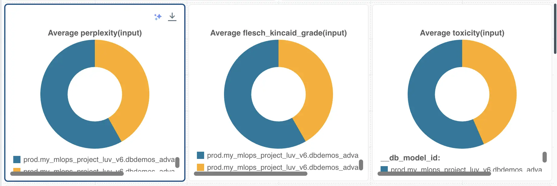
These three pie charts represent metrics assessing changes over time between two versions of a model: an older version (indicated in blue) and the latest version (shown in yellow). The metrics presented are average perplexity, Flesch-Kincaid readability index, and toxicity level. The color coding suggests that the newer version of the model shows improvements (less) compared to the older version (more).

The interpretation of these charts can be instrumental in evaluating the evolution of the model in terms of complexity, readability, and safety. A decrease in perplexity may indicate that the model’s predictions have become more predictable or contextually appropriate, which can enhance user satisfaction. Improvements in the Flesch-Kincaid readability score suggest that the text generated by the model is easier to read and understand, making it more accessible to a broader audience. A reduction in toxicity levels is critical, as it reflects a safer interaction environment for users, minimizing the risk of generating harmful or inappropriate content.

These metrics not only demonstrate the model’s enhancement in generating more user-friendly and ethical content but also serve as indicators of the overall health and security of the system. Monitoring these changes can help in early detection of anomalies that might indicate potential security breaches or degradation in user experience.

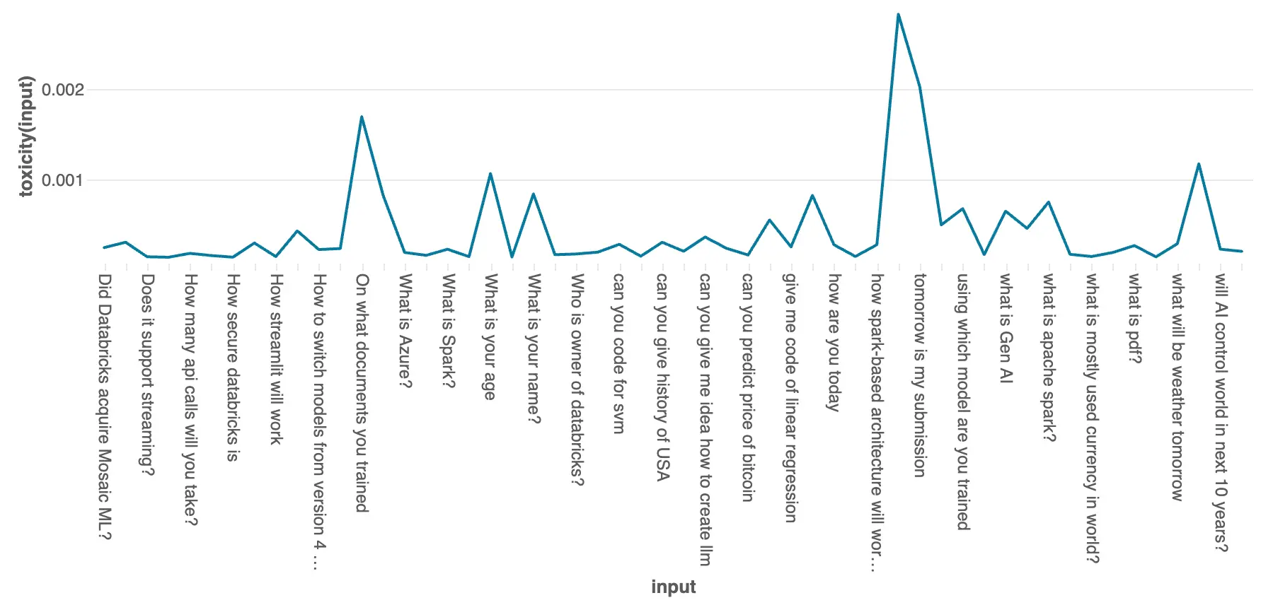
As you can see below, the graphs show the line chart for prompts used by the users versus the toxicity score. This can help us to generate flags for toxic inputs and do further prompt engineering to make the bot more ethical and user-friendly.

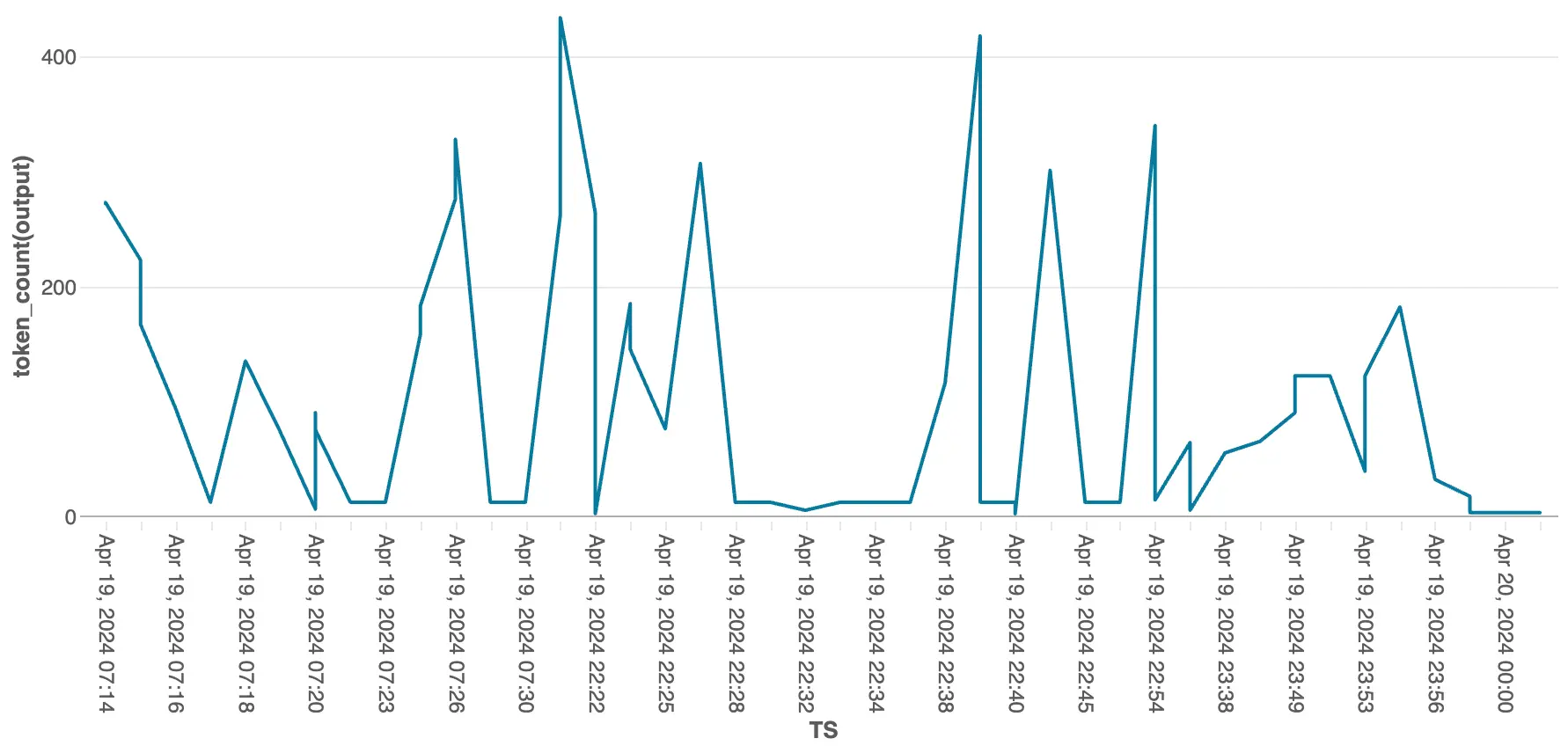
This graph shows the token output by our model over time, this helps to see flags and also for cost tracking. This graph can be further analyzed by tracking the usage over a specific period of time. This helps to solve the latency issue.

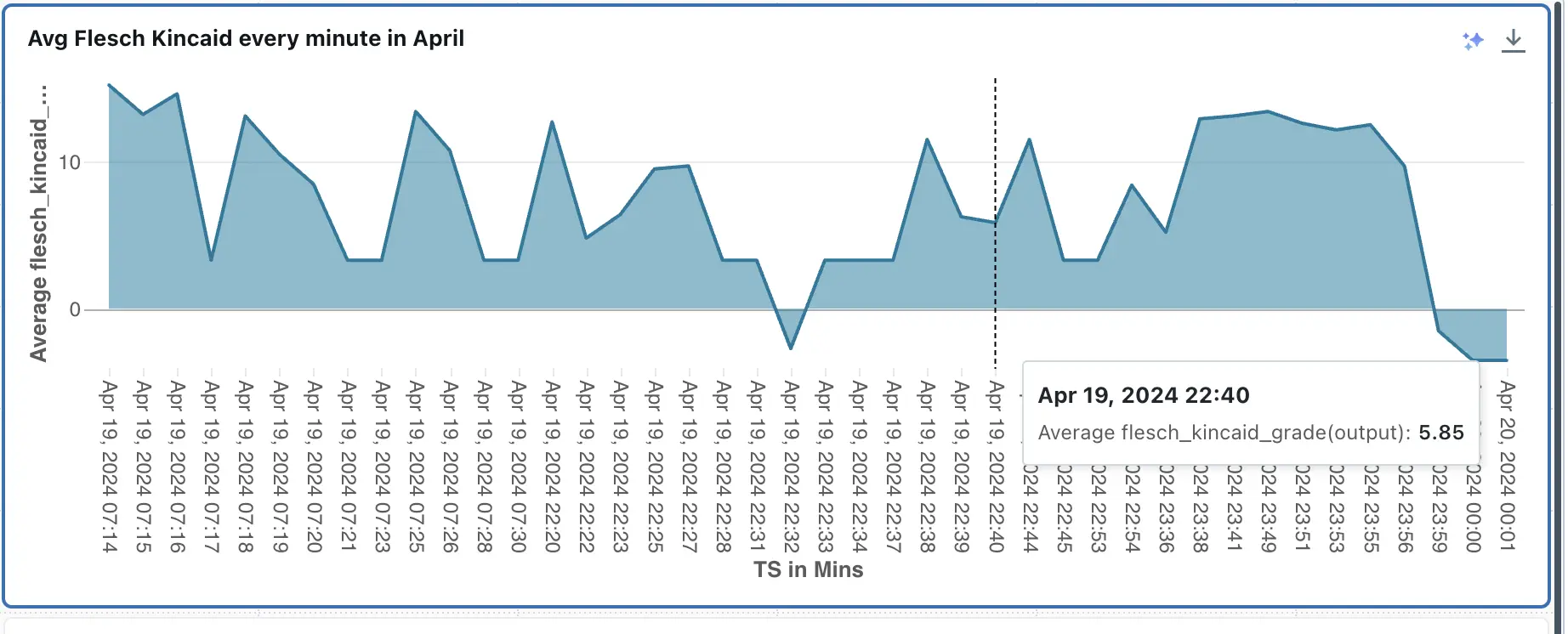
Here you can see the Flesh Kincaid score for every minute the model is being used in the month of April. This score is for checking the readability of the model. For understanding the metric better, refer.