Table of Contents
1. Deep Learning Model
1.1 Model Overview
The model used is a Convolutional Neural Network (CNN) designed for a multi-class classification task, specifically for speech emotion recognition. The network’s architecture consists of multiple convolutional layers followed by pooling and batch normalization layers, and it concludes with fully connected (dense) layers for classification.
Layer details: Convolution layers, MaxPooling, Dropout for regularization, and Dense layers for classification.
Activation functions: ReLU for hidden layers and softmax for output layer to classify emotions.
1.2 Model Architecture
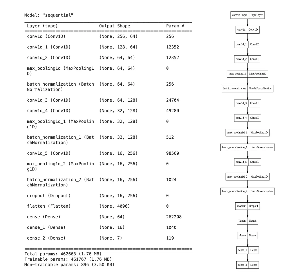
Here’s a detailed breakdown of the architecture:
- Input Layer:
- Takes input data of shape (inp_shape, 1).
- First Convolution Block:
- Convolutional layer with 64 filters, kernel_size=3, strides=1, and ReLU activation.
- Convolutional layer with 64 filters, kernel_size=3, strides=2, and ReLU activation.
- Convolutional layer with 64 filters, kernel_size=3, strides=2, and ReLU activation.
- MaxPooling layer with max pooling=2, strides=1.
- BatchNormalization layer.
- Second Convolution Block:
- Convolutional layer with 128 filters, kernel_size=3, strides=1, and ReLU activation.
- Convolutional layer with 128 filters, kernel_size=3, strides=2, and ReLU activation.
- MaxPooling layer with max pooling=2, strides=1.
- BatchNormalization layer.
- Third Convolution Block:
- Convolutional layer with 256 filters, kernel_size=3, strides=2, and ReLU activation.
- MaxPooling layer with max pooling=2, strides=1.
- BatchNormalization layer.
- Dropout layer with dropout_rate=0.2.
- Fully Connected Block:
- Flatten layer.
- Dense layer with 64 units and ReLU activation.
- Dense layer with 16 units and ReLU activation.
- Output Dense layer with 7 units (number of classes) and softmax activation.
1.3 Training Process
- Data Preparation:
- Data is loaded and preprocessed from parquet files.
- Labels are one-hot encoded.
- Features are expanded to include an additional dimension for compatibility with the Conv1D layers.
- Hyperparameter Tuning (Optional):
- Uses Optuna to perform hyperparameter tuning.
- Tunable parameters include number of filters, kernel size, pooling size, and dropout rate.
- Training Configuration:
- Optimizer: Adam
- Loss Function: Categorical Crossentropy
- Metrics: Accuracy
- Callbacks:
- ReduceLROnPlateau: Reduces learning rate when a metric has stopped improving.
- EarlyStopping: Stops training early if the validation loss does not improve for a certain number of epochs.
- LoggingCallback: Custom callback to log the epoch end details.
- Model Fitting:
- Trains the model using the training dataset and validates it on the validation dataset.
- Uses the configured batch size and number of epochs.
- The model’s performance metrics are logged.
- Model Checkpointing:
- The trained model is saved to disk in a specified format.
1.4 Optimizers and Training Details
- Optimizer: Adam
- Adam is a popular optimization algorithm in deep learning due to its adaptive learning rate properties.
- Loss Function: Categorical Crossentropy
- Suitable for multi-class classification tasks.
- Metrics: Accuracy
- The model is evaluated based on the accuracy metric.
1.5 Model Training Pipeline Workflow
- Initialization:
- Load configuration parameters from params.yaml.
- Initialize one-hot encoder and Google Cloud credentials.
- Data Preparation:
- Load training and validation data.
- Encode labels and expand feature dimensions.
- Save processed data and encoder for future use.
- Model Definition:
- Define the CNN architecture as described above.
- Hyperparameter Tuning (if enabled):
- Perform hyperparameter tuning using Optuna.
- Update model parameters based on the best hyperparameters found.
- Training:
- Compile the model with the Adam optimizer, categorical crossentropy loss, and accuracy metric.
- Train the model with early stopping and learning rate reduction on plateau callbacks.
- Log training duration and metrics.
- Saving:
- Save the trained model and log relevant details.
2. Orchestrating Workflows using Airflow
In this project, orchestration of workflows is managed through Apache Airflow, a powerful tool that schedules and manages complex workflows. For local development, Airflow is containerized using Docker, providing a flexible and isolated environment for testing different workflows without affecting the host system. In production, these workflows are scaled and managed through Google Cloud Composer, a managed Airflow service that integrates seamlessly with other Google Cloud services, enhancing our deployment’s efficiency and reliability.
2.1 Setup for Docker
Docker setup involves creating a Dockerfile that specifies the Airflow version and configuration settings appropriate for the project’s needs. Docker-compose files are used to define services, volumes, and networks that represent the Airflow components such as the web server, scheduler, and worker
2.2 Initial Setup for AirFlow
Setting up Airflow involves defining Directed Acyclic Graphs (DAGs), which outline the sequence of tasks and their dependencies. Each task is represented by operators, such as PythonOperator or BashOperator, which execute specific pieces of code necessary for the workflow.
2.3 General Runs of Airflow insider Docker Containers
Running Airflow inside Docker involves spinning up the containers using docker-compose, which reads the docker-compose file to start services defined for Airflow. This encapsulated setup ensures that all dependencies and configurations are consistent across different development environments.
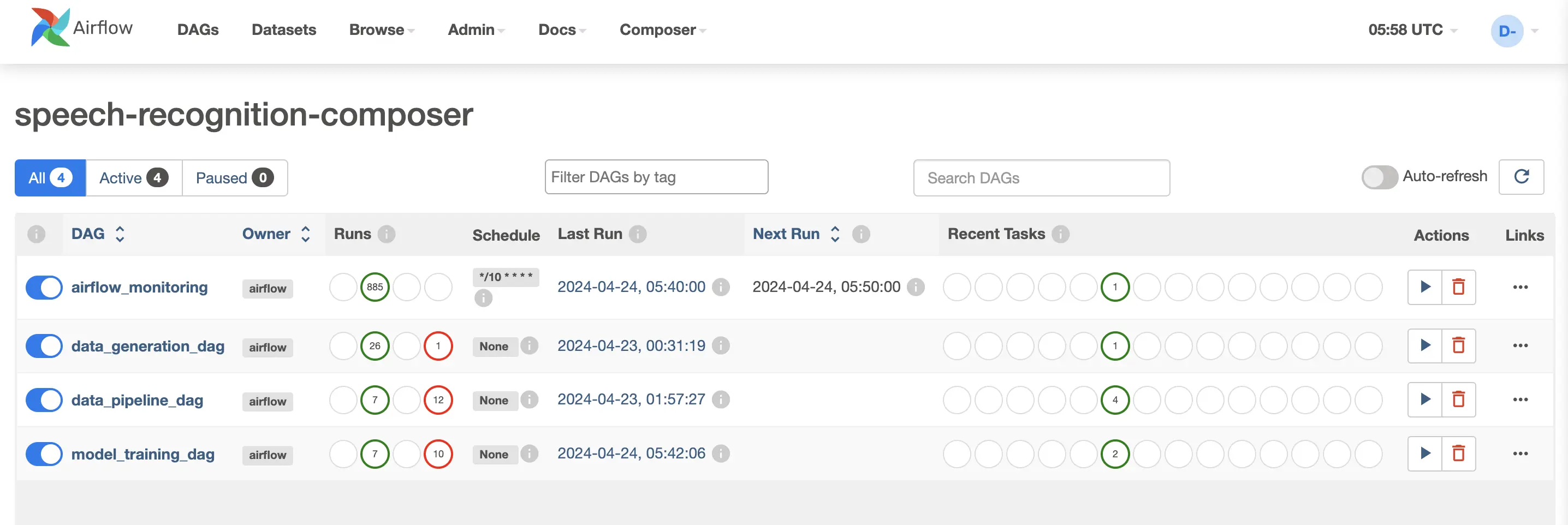
2.4 Operating through UI inside Airflow
Airflow’s web-based UI allows users to monitor and manage their workflows. It provides detailed visualizations of pipeline dependencies, logging, and the status of various tasks. The UI is crucial for troubleshooting and understanding the behavior of different tasks within the DAGs.